EDdy Dynamics,
mIxing, Export, and Species composition
(EDDIES)
Project Summary and Cruise Logistics
Updated August 12, 2003
Contents:
1. Hypotheses
2. Scenarios
3. Objectives
4. Selection of the target eddy feature
5. Sampling operations
6. Measurements
7. Berthing
8. Related projects and proposals
9. Project timeline
Appendices
A. Detailed sampling information: Café Thorium
B. Detailed sampling information: Siegel
C. Detailed sampling information: Hansell
1. Hypotheses
Prior results have documented eddy-driven transport of nutrients into the euphotic zone and the associated accumulation of chlorophyll. However, several key aspects of mesoscale upwelling events remain unresolved by the extant database, including: (1) phytoplankton physiological response, (2) changes in community structure, (3) impact on export out of the euphotic zone, (4) rates of mixing between the surface mixed layer and the base of the euphotic zone, and (5) implications for biogeochemistry and differential cycling of carbon and associated bioactive elements. This leads to the following hypotheses concerning the complex, non-linear biological regulation of elemental cycling in the ocean:
H1: Eddy-induced upwelling, in combination with diapycnal mixing in the upper ocean, introduces new nutrients into the euphotic zone.
H2: The increase in inorganic nutrients stimulates a physiological response within the phytoplankton community.
H3: Differing physiological responses of the various species bring about a shift in community structure.
H4: Changes in community structure lead to increases in export from, and changes in biogeochemical cycling within, the upper ocean.
2. Scenarios
There are several scenarios in which this chain of hypotheses could be linked or broken. These include, but are not necessarily limited to, the following:
S1: Nutrient input to the euphotic zone simply increases the rate of production by the background species assemblage dominated by picoplankton; impacts on biogeochemical cycling are nil.
S2: Increased nitrate availability stimulates a bloom of diatoms; silica-rich organic material produced in the bloom sinks rapidly out of the euphotic zone once the nutrients are exhausted.
S3: Shoaling isopycnals transport DIP closer to the surface, facilitating nitrogen fixation by Trichodesmium or perhaps vertically migrating diatoms with symbiotic bacteria; nitrogen-rich organic material produced during the bloom is exported primarily in dissolved form.
S4: The eddy feature accommodates a change in community structure and biomass of consumers that produce rapidly sinking particles.
3. Objectives
The following objectives are designed to test hypotheses H1-H4 and distinguish between the scenarios S1-S4 in which the chain of hypotheses are linked or broken.
O1: Measure the enhancement of inorganic nutrient availability brought about by eddy-induced upwelling.
O2: Measure the phytoplankton physiological response to increased nutrients.
O3: Assess shifts in species composition associated with the eddy disturbance.
O4: Quantify the impact of the eddy disturbance on upper ocean biogeochemical cycling: measure elemental inventories, primary production, and export.
O5: Assess the interaction between eddy-driven isopycnal transport processes and diapycnal fluxes in and below the mixed layer (quantifies the reversibility of the eddy-induced transport; specifically, how is the oxygen anomaly “left behind” and eddy-driven new production event).
4. Selection of the target eddy feature
Real-time analysis of altimetric observations will provide maps of the eddy field prior to and during our sampling operations.
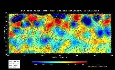
As far as we know, there are three different types of mid-ocean eddies in the Sargasso Sea: cyclones, anticyclones, and mode-water eddies (MWEs). Cyclones and MWEs are of interest to this project, as both tend to displace upper ocean isopycnals toward the surface, causing nutrient input into the euphotic zone. Whereas cyclones are identifiable in satellite altimetry by virtue of their negative sea level anomaly (SLA), MWEs are not distinguishable from anticyclones on the basis of altimetry alone because both result in positive SLA. In principle, satellite-based SST could distinguish these two, as anticyclone and MWEs would be characterized by warm and cold SST anomalies, respectively. However, given the paucity of reliable SST imagery in the Sargasso Sea during summer, we will likely have to rely on in situ measurements to unequivocally distinguish MWEs from anticyclones.
Eddy age is another key issue. Whereas an intensifying cyclone will have upwelling in its center, the isopycnals in the interior of a decaying cyclone will be downwelling. The earlier phase of the eddy’s lifetime will be when nutrient injection and the associated biological response occur.
Summary of desirable characteristics for the target eddy:
1. Young
2. Strong
3. Intensifying
4. Chemical impact discernible in real time (optical NO3 sensor)
5. Biological impact discernible in real time (fluorometry, microscope counts, VPR?)
6. Cyclone versus MWE?
a. unequivocal satellite determination favors cyclones
b. trapping of near-inertial motions and possible enhanced mixing favors MWEs
c. some of the big events at BATS have been MWEs
Jenkins (1988) Summer 1986 event
McNeil et al. (1999) July 1995 eddy
7. Proximity to BBSR: must be within 1 day’s steam for Weatherbird II
Clearly, it will behoove us to sample several eddies during the first survey cruise prior to making a decision about which eddy we wish to spend the rest of the summer in.
5. Sampling operations
Once the target feature is chosen, intensive sampling will begin:
Oceanus: 2 snapshots per “Survey Cruise”
Weatherbird II: 2 sections per “Section Cruise”
Timeline:
6/10
– 7/2 7/5 – 7/20 7/23 – 8/9 8/12 – 8/27
Oceanus Survey 1 Tracer 1 Survey 2 Tracer 2
Weatherbird II Sections 1 Sections 2
Note that five days of ship time (originally requested for a test cruise in April) have been added to the first survey cruise. This shifts the timing of all subsequent cruises from an earlier version of the schedule.
6. Measurements
Remote sensing
Altimetry, ocean color, SST McG/Siegel
Oceanus Surveys
XBT McG
ADCP McG
CTD + FRRF + Optical NO3 McG/Falko/Siegel
Niskin water sampling
HPLC
NO3, PO4, SiO2
POC, PON
Helium/Tritium Jenkins
Microscope counts Falko
Bio-optics (casts) Siegel
Bio-optical drifter Siegel
VPR? Davis
Weatherbird II Sections
NO3, PO4, SiO2; HPLC; POC, PON Bates 16-20 depths; 24-place rosette
14C Productivity Bates
Sediment traps (150m) Bates
TCO2, pCO2, O2 Bates
DOC, DON, DOP, δ15N(PON) Hansell
Thorium-based export Buesseler 2hr casts edge/middle/center
FRRF Falko
Oceanus Tracer Cruises
SF6 Ledwell ship available half time
Gliders
CTD, fluor., opt. backscatter, PAR Fratantoni
Notes:
Will there be a sediment trap outside the eddy? Can BATS serve as the control?
FRRF work at night; can dark adapt (1 hour delay)
Falkowski may bring along a FlowCAM
Niskin sampling depths:
Prior work used 0,20,40,60,80,100,120,140,200,300,500,700 (12 depths)
Should we increase resolution near the base of the euphotic zone?
Bottle sample inventory
Oceanus: 2 cruises x 2 snapshots x 25 stations x 12 depths = 1200 samples
Weatherbird II: 2 cruises x 2 sections x 7 stations x 12 depths = 336 samples
Total: 1536 samples
Utilizing down time on Ledwell cruises
Sampling sled stays attached to hydro wire
Sample 4-5 hours; process 4-5 hours [ship available during processing]
Oceanus salt bottles to be stored aboard ship and run upon return to WHOI; experience suggest storage period of up to one year is acceptable, provided that bottle neck and cap are dried thoroughly prior to closure.
Logistics:
Ship gear to Bermuda or pack on Oceanus?
7. Berthing
Oceanus Survey Cruises [capacity 14-18]
McGillicuddy 6
Falkowski 2
Siegel 1
Jenkins 2
Fratantoni 2-3
[Davis] 2
[Brzezinski] 2
[Armbrust] 1-2
Oceanus Tracer Cruises [capacity 14-18]
Ledwell 6
Weatherbird II [capacity 10]
Bates 3*
Hansell 1*
Buesseler 2
Falkowski 2
[Carlson] 1-2
[Steinberg] 1-2
*These 4 people comprise the hydro team that will run 12 on / 12 off shifts.
8. Related Projects and Proposals
Fratantoni Gliders
Davis VPR
Oakey/Ledwell Finestructure
Steinberg Zooplankton net tows
Carlson prokaryotic community structure and DOM dynamics
Armbrust genetic diversity in eukaryotes
Shipe/Brzezinski N and Si uptake
Benitez-Nelson et al. Hawaiian Eddy Project
9. Project timeline
2003
July 1 Start Date
July 23 First PI meeting, Woods Hole
2004
February Second PI meeting, ASLO/TOS Conference, Honolulu
Summer Field Work
2005
Winter PI meeting: analysis of ’04 and planning for ‘05
Summer Field Work
2006
Winter PI meeting: synthesis and manuscript preparation
June 30 End date
Appendix A: Detailed sampling information - Café Thorium
4 Liter sampling plan
- Approximate number of 4 liter samples: 120-140/cruise
This plan is based on 10-12 point profiles collected at each station.
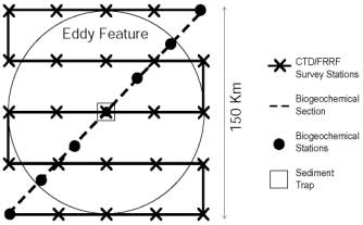
- 7 stations to be sampled during BGC section 1 will include: 2 out stations, 2 edge stations, 2 middle stations, 1 center station. 6 stations sampled on BGC section 2 include: 1 out station (excluding the most recent out station), 2 edge stations, 2 middle stations, 1 center station.
- 1 deep water (4000 meter) calibration cast is required. 10 samples for 234Th calibration collected.
- We estimate a 4l sample collection rate of 20/day.
- Approximately 3 days are needed for sample processing. Will require 2 days at the dock to finish processing.
- All beta counting will be performed back at WHOI.
- In ships lab, rack space for filtration apparatus will require 4x8 feet of wall space. (We are requesting the aft section of the WB II main science lab. See deck layout)
- Berthing requirements: 2 persons on each leg. (Need to find 1 person for June ’04 and July “04 cruise)
- Jan ’05: recovery chemistry at WHOI (Need 1 person for lab work: Claudia student?, Pinghe Cai?)
Pump sampling plan
- A total of 8 stations sampled BCG Sections 1 and 2. Section 1: 2 out stations, 2 edge stations, 1 eddy center. Section 2: 1 eddy center, 1 edge, 1 out
This plan is based on 4 point profiles collected at each station.

- Casts will consist of 4 pumps deployed simultaneously for 2 hours, or 2 casts with 2 pumps deployed for a total of 4 hours. Total volume of 500l at 8 l/min. 1 hour total deployment/recovery time.
- Wire time required: 16 hours w/4 pumps, 32 hours w/2 pumps.
A request has been made to have 4 pumps available so as to minimize wire time requirements.
· Pump deployment will require separate hydro-wire and winch.
· Each pump will be fitted with a 142 mm 54um screen followed by a 1.0 um quartz filter. Total of 64 particulate samples for C/Th analysis and counting. (32 silver filters/cruise)
Other:
· Will there be a drogued PITS traps deployed by BATS team?
Should a trap be shipped back from Hawaii for the July ’04 cruise?
· Counting: 54 um samples need to be counted first. (Typical BATS activity for these samples is as low as 0.6 cpm) 3 days counting time required for all silver filters.
· 14 days required for counting 4l samples. All counting finished in 14-16 days from collection date. (BATS samples are around 3 cpm after 10 days)
Appendix B: Detailed sampling information – Siegel
The UCSB group will make three field measurements in support of EDDIES 2004.
1. Spar array between the two survey cruises
2. Profiling spectroradiometery casts to characterize UW light field in and around the eddy from the survey cruises
3. Autonomous NO3 sensor on the survey CTD package
The spar array will be made up of 7 SBE-39s (temperature loggers with 2 millidegree accuracy) and 3 WETLabs chl-fl/backscatter sensors (ECO-FL-NTUSB; http://www.wetlabs.com/Products/eco/flntu.htm). There may be more instrumentation deployed depending on budgets, etc. The spar will have a surface light and an ARGOS transmitter (maybe two) and will be drouged with a holey sock at the depth of the tracer release. Dave Menzies can handle this and will be on both cruises; modulo some help on deck deploying and retrieving.
The profiling spectroradiometer is a Satlantic SPMR system with 12 or so channels of downwelling irradiance, upwelling radiance, chl-fl and temperature on the fish and a surface sensor for measuring incident downwelling irradiance. The SPMR is a hand-lowered instrument that is designed to minimize ship shadows. There will be a small hand reel for the cable that needs to be bolted to the deck. We want casts from daylight hours (preferably 0900 to 1600) and normally deploy from the stern with stern facing the sun. The deployment takes two people minimally; one running the aquisition computer and one handling the kevlar cable. With Dave M going alone from UCSB, we will need some help with this (either on deck or in the lab). The deployments take less than 20 minutes per station. The surface sensor needs have an unobstructed view of the sun, be able to run cables into the lab computer and have a seawater supply via a garden hose (for cooling). We've done this on the Ron Brown before and will on the Knorr this fall. The computer should be near access to the fantail and we may want to use radios to communicate from lab to deck.
The last is that we'll be responsible for the care and feeding of the optics sensors on the survey CTD and the UCSB NO3 optical nitrate sensor. This should be easy but will require us to do air cals of the transmissometers, etc.
I figure we will need 3 to 4 feet of lab space for all of this although a good deal of storage for the spar equipment. I'm not sure of hazmats at this time, but I think we'll have ethanol for cleaning optical windows.
Appendix C: Detailed sampling information – Hansell
Water budget:
DOC 100 ml
DON 100 ml
DOP 200 ml
Del 15N PON (4 L, but only at the shallowest depths). Perhaps we could take some of this with bucket casts, or perhaps these samples should come from the survey.