The SeaWinds on QuikSCAT 

The SeaWinds on QuikSCAT Level 3 data set consists of gridded values of scalar wind speed, meridional and zonal components of wind velocity, wind speed squared and time given in fraction of a day. Rain probability determined using the Multidimensional Histogram (MUDH) Rain Flagging technique is also included as an indicator of wind values that may have degraded accuracy due to the presence of rain. Data are currently available in Hierarchical Data Format (HDF) and exist from 19 July 1999 to present time. 

The Level 3 data were obtained from the Direction Interval Retrieval with Threshold Nudging (DIRTH) wind vector solutions contained in the QuikSCAT Level 2B data and are provided on an approximately 0.25° x 0.25° global grid. Separate maps are provided for both the ascending pass (6 AM LST equator crossing) and descending pass (6 PM LST equator crossing). Scaling factor * 100 has been applied to the wind speed (m/sec). By maintaining the data at nearly the original Level 2B sampling resolution and separating the ascending and descending passes, very little overlap occurs in one day. However, when overlap between subsequent swaths does occur, the values are over-written, not averaged. Therefore, a SeaWinds on QuikSCAT Level 3 file contains only the latest measurement for each day. This product is also referred to as JPL PO.DAAC product 109. 

 Grid Description:

The QuikSCAT Level 3 data set is on a simple, rectangular grid of 1440 columns by 720 rows. Therefore, a grid element spans 0.25 degrees in longitude (360/1440) and latitude (180/720). Latitude and longitude coordinates are assigned to each grid element based on its center. To calculate the longitude and latitude of a grid point, the following equations can be used:

                                            lon[i] = (360./XGRID) * (i+0.5)
                                                                                                      for i=0...XGRID-1
                                            lat[j] = (180./YGRID) * (j+0.5) - 90.
                                                                                                      for j=0...YGRID-1

    where:
                                             XGRID=grid elements in the x-direction (1440)
                                             YGRID=grid elements in the y-direction (720)

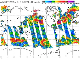
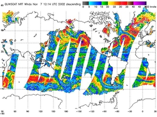
As shown by the above formulas, the latitude and longitude of the center of the first grid cell of each QuikSCAT Level 3 scientific data is -89.875° North (89.875° South) and 0.125° East. The latitude and longitude of the final grid cell of each data set is centered at 89.875° North and 359.875° East (0.125° West). 

The following map displays the ocean surface winds at a 10m height from ascending and descending  satellite passes as processed by NOAA/NESDIS, from near real-time data collected by NASA/JPL's SeaWinds Scatterometer aboard the QuikSCAT. 

  Flag file Description:

asc_wvc_count: distinguishes NULL values from zero value of wind speed in  the ascending pass data. If asc_wvc_count is 0 in a given cell, wind retrieval did not take, and wind speed values are NULL in that cell. If asc_wvc_count is 1, wind retrieval occurred, and a 0 value of wind speed indicates a measurement of 0 m/s.

 Data and processing:

 The objective of this study is to get a wind product with realistic high temporal/spatial resolution and to compare this product (wind field, wind stress and wind stress curl)  to mesoscale fields in the Sargasso Sea.

 The Atlantic Ocean from 28°N to 36°N and from 60°W to 70°W ("large" domain) was chosen as the region to generate QSCAT daily wind fields. QSCAT data began on 19 July 1999, and extended (currently) up to 30 June,  2002. The coverage of QSCAT is extensive, giving a continuous swath of 1,800 km, providing wind vector measurements over 90% of the ice-free global oceans each day.   Despite the high quality and excellent
coverage that QSCAT data provided, the data contain spatial gaps that need to be filled before these observations can be easily utilized.

 A different technique was used to create regularly gridded daily wind maps from QSCAT ( or NSCAT ) scatterometer observations, see fo example,  Zeng and Levy (1995), P. Polito et al (2000), W.T. Liu et al (1998, 2000), M. Bourassa et al (1999).  Space based wind measurements either have to be subjected to averaging within a certain temporal and spatial bin, or be interpolated with some type of smoothing or filtering. The simplest way to form a daily gridded winds is just to take an average of the ascending and descending data for the same day. But the main problem in such mapping is to prevent the appearance of swath patterns in wind fields is still remains. The other hand, space-time interpolation and filtering result in smoother wind field but reduce the energy it contains.  A proper interpolation of QSCAT data is intended to alleviate this drawback, and, what is very important, retains greater energy content at high wavenumbers. 

Let's overview briefly a few more methods that have been used recently to process QSCAT/NSCAT data.

 1.   The correlation-based interpolation method (P. Polito et al, 2000) uses a sequence of regularly gridded maps of a wind speed component as input. These maps may have data gaps, indicated by a numerical flag, which requires interpolation. The three-dimensional autocorrelation coefficient matrices derived directly from daily bin averaged maps in a regular grid  used for the interpolation onto the same grid. The autocorrelation matrices are continuously updated in space and time.

The algorithm starts by estimating the autocorrelation coefficients in the volume limited by the maximum zonal, meridional and temporal lags which are set 4°,  3°, and 2 days. The autocorrelation coefficients are calculated at each grid point using spatial (x_l,y_l) and temporal (t_l)
lags.  Each interpolated point is obtained from the weighted average of N_s selected points using the autocorrelation coefficients as weights.
The criteria to select data points and weights are in the averaging process have two adjustable parameters: the maximum number of points N_p, and the minimum correlation threshold c_min. The autocorrelation matrix is then sorted so that up to N_p coefficients larger then c_min are used.
If less then a minimum number of points (n_p=5) remains after the selection criteria are applied, a canonical correlation matrix is used instead of the estimated one. The coefficients of the canonical correlation are calculated by

                                   C(x_l, y_l, t_l) = 1/( 1 + sqrt( 2 x t_l² + 0.5 x_l² + 0.5 x y_l²))
This is  a symmetric inverse-distance function that has decay scales similar to the average of those inferred from ECMWF winds.

 2.   The approach developed in Bourassa et al, 1999, retains the dominance of winds observed on the day in question, and it also allows for a relatively smooth transition into regions where there were no observations, or smoothly fill the gaps. First of all, a binning procedure was applied to the 25-km resolution NSCAT winds. The bin size was chosen 50 km to include sufficient observations. Then the  weighting procedure analogous to a weighted vector average of 1-, 2-, 4-, and 8-day averages was applied to binned winds. Each of this averaging periods was centered on 1200 UT of the day in question. The weighting mechanism is designed to favor observations in the short averaging periods. The 8-day averaging period was sufficiently long that there are observations in each grid box.  The effective averaging window is reduced through a weighted average u₄* of the 8-day u₈ and 4-day u₄ fields. The effective averaging window is the further reduced by averaging the product u₄* with 2-day and 1-day averages. The key equations are

                                         u₄* = (n₄ x u₄ + n₈ x u₈)/(n₄+n₈),    u₂* = (n₂ x u₂ + n₄* x u₄*)/(n₂+ n₄*),
                                         u₁* = (n₁ x u₁ + n₂* x u₂*)/(n₁ + n₂*), 
                                         n₄* = (ß x n₄ + n₈)/( ß+ 1), n₂* = (ß x n₂ + n₄)/(ß+1),

where n is the number of observations in a given cell. Increasing the value of the weighting parameter ß sharpens the fit to u1 at the expense of smooth fields near swath edges. It was found a value of ß=5 to be optimal.

 3.   Another one method developed by Timothy Liu et al, 1998, objectively interpolates NSCAT winds by  the method of successive corrections. The interpolation scheme starts with the NSCAT monthly bin-averaged  field as an initial guess field. Then, NSCAT observations within the radius of influence (R)  and the period of influence (T) of the chosen grid point are used to make corrections iteratively. The value of T was chosen 1.5 days,  and R decreases from 10 grid-spacing to 1 during the 5 successive iterations. The contributions of observations to the correction term were weighted differently according to their positions relative to the grid point under analysis. Observations were screened out if the difference between them and the interpolated value of the analyzed field exceeds the maximum allowable error (E). E decreases from 50 m/sec to 3 m/sec over the 5 iterations.

The key point for the successive corrections is imbedded in the equation

                                                                                          ugⁿ⁺¹ = ugⁿ + ß Cn

where ß is a weighting factor and Cⁿis the correction term representing the impact from the observations. To produce a map of a particular time T, the value on each grid point is initialized by the NSCAT monthly bin-averaged  field. 
To figure out the correction term on the n-th iteration, guess fields ugⁿ  were used to calculate the guess field value ug _sⁿ  at location "s" where scatterometer data were obtained. The interpolation guess field value ug_sⁿ  is given by the 9-point Lagrangian interpolation formula:
                                                                                             _{i=I+1, j=J+1}
                                                                         ug_sⁿ  = E w ug^{n
                                                                                             i=I-1, j=J-1}
where (I,J) is the grid point closest to location "s" and w is the weighting function given by 
                                                                            _{k=I+1, k~=I                        l=J+1, l~=J}
                                                                         w = P (x - x_k) / (x_l - x_k) P (y - y_l) / ( y_J - y_l)
                                                                            ^{k=I-1, k~=I                       l=J-1, l~=J}
Here (x,y) represents the coordinates of location "s". 

Next the error E_s^n, the difference between the actual measured scatterometer value us at location "s" and the guess value interpolated from the analyzed field at the same location, is computed:

                                                                                    E_sⁿ = u_s - ug_sⁿ

Observed data were rejected if this error value exceeds the maximum allowable error (E_max) as given in  table (not shown). This error limit is a decreasing function of iteration passes, allowing increasing confidence in the analyzed field with each successive iteration.

The error function  E_sⁿ is used to correct the guess field  value on grid points for the (n+1)-th iteration. The correction term is given by

                                                                                     Cⁿ = E W_sⁿ   E_sⁿ / E W_s^{n
                                                                                                s            s} 
where the summation is over all observations within the radius of influence, Rn.  W_sⁿ  is a weighting factor defined as W_sⁿ =w_n(d) b(t). 
For each wind map, the correction process was performed four times successively.

Of course, the advantages and disadvantages of each the above listed methods depend on the application of the wind field product.

 Wind field computation:

 The ascending and descending data were averaged together to form daily composites of  wind field with no smoothing. Then, these maps were interpolated onto the T/P diamond domain in same manner as it was described above, and used in the next analysis. 

Also, the relatively simple binning and weighting method of Bourassa et al, 1999  has been used to produce daily wind field and its derivatives (e.g., curl and divergence) over the T/P diamond domain. First, daily winds were produced for  the "large" domain, then cubically interpolated onto the T/P diamond.  The resulting fields are used to examine  a possible connection of surface winds with  mesoscale features observed at BATS site. 
 

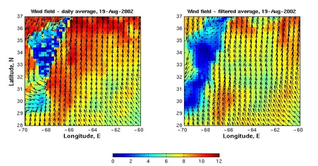
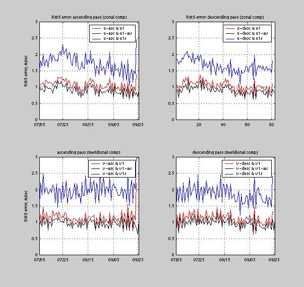
 Results.

 a.  daily averages from ascending /descending passes

 An example of daily averages  mapping  presented in  fig. 1a. -- how the daily composites have been created,  fig.1b  -- daily winds,  and fig.1c -- daily wind stress curl.   The whole data set can be scrolled day by day using   la_wind_99_02.fli   (winds), or  la_curl_99_02.fli  (wind stress curl) movie.

 b. daily averages from space-time smoothing

 As an  alternative to simple averaging described above, the space-time filtering was applied to daily averages to remove small-scale variability and noise. The running 8 points ( 8 days) gaussian filter was used to smooth the time-series in each pixel. Then the running box ( 5 x 5 points, or 1^o x 1^o ) gaussian filter was applied to each image. An example of such smoothing displayed here -- la_wind_ts_filt.fli.

 c. description of the tests and error analysis for the  method of Bourassa et al

 The NSCAT wind  fields from July 1 through September 30, 2002 were used to test  a smoothing technique. The figure below presents results from test comparing results from daily composites and the Bourassa et al, 1999, algorithms ( also, scroll day by day results of this test using  av_filt_12.fli   movie ). 

 A little loss of information is clearly seen in smoothed map. Same time, zone of low winds is  now more accurately described due to corrected ambiguity selection.
A rms difference between the ascending/descending original wind fields,  binned 1 day  winds u₁,  smoothed 1 day winds u₁*, and daily composites u₁^d  presented in  fig. 2  (separately for zonal and meridianal components). For the region examined herein (70^oW to 60^oW, 28^oN to 37^oN), there is a rms difference of ~ 1.0 m/sec in the east-west wind component u, 1.1 m/sec in the north -south wind component v (comparing to 1 day binned and composites).  It was found that in case of 1 day smoothed winds (u₁* ) this rms difference increased to 1.7 m/sec and 1.8 m/sec correspondingly. 
Next plot ( fig. 3 ) shows correlation coefficient calculated between different pairs of zonal wind component. The lowering of the correlation coefficient is clearly seen in all pairs where smoothed 1-day winds u₁* are presented. Simple bin-averaged winds (u₁) and daily composites (u₁^d) do not show any significant loss of correlation. Correlations between data from individual ascending/descending passes, and that received as a result of  averaging/filtering data processing, just represent the  effect of  time-averaging when data from ascending and descanding passes  are getting together.

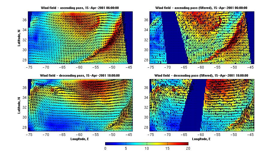
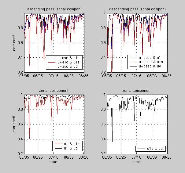
 d. mapping individual ascending/descending passes

 In some cases when analyzing simultaneously satellite data like SeaWiFS imagery, a corresponding synoptic scale wind data are required.  The main problem related to getting daily scatterometer data is that the observational tracks from different times (passes) intersect, often  with substantial changes in wind pattern occurring between the observations. Simple averaging would result in spurious wind curl and divergence which then can lead to incorrect conclusions. To avoid  such situation a simultaneous wind data from individual ascending/descending passes have been mapped and analyzed.

 As a first step, gaps in wind field were filled using 2D cubic interpolation and compared to the original data. An example of such interpolation and comparison is shown below. To scroll data between April 1, 2001 and May 10, 2001 click  here /wind #1/.

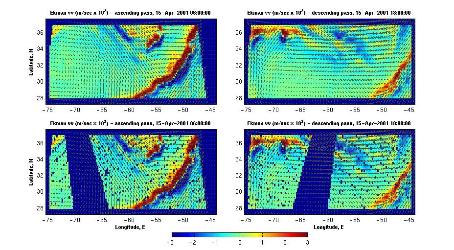
 Next plot displays corresponding Ekman vertical velocity field during same period of time.

 To scroll data between April 1, 2001 and May 10, 2001 click  here /wind #2/.
 Next plot displays combined wind speed/ekman vertical velocity plot. The only difference between the plot displayed above and the current one is that the current plot was smoothed with the 150 x150 km^2 averaging filter.

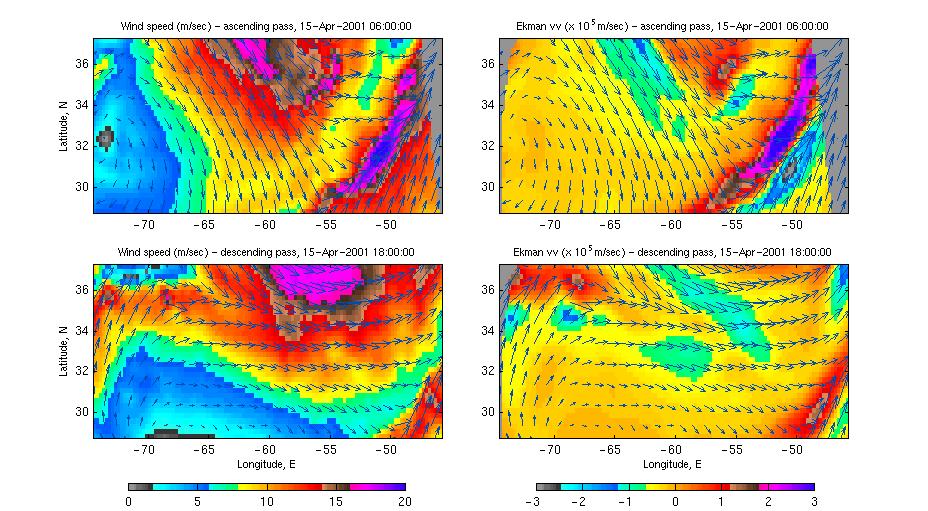
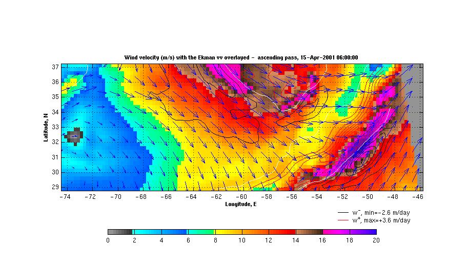
 Finally, next 2 plots display  wind field with the Ekman vertical velocity overlaid.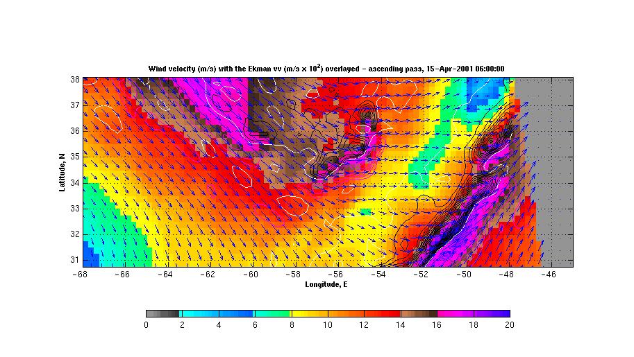

 or same field with max/min values vertical velocity displayed (larger domain).

 To scroll data between April 1, 2001 and May 10, 2001 click  here /wind # 4/ ,or  here  /wind # 5/ .
 

                                                                                        Analysis of the combined SeaWiFS, AVHRR and QuikSCAT data.

                                                                                                                                                  SeaWiFS

April 23, 2001

April 25, 2001

April 28, 2001

May 4, 2001

                                                                                                                                      SeaWiFS + SLA

AVHRR

April 23, 20:43	April 25, 20:19	April 28, 17:39	May 3, 17:01	May 3, 20:24
May 4, 06:50	May 4, 08:48	May 4, 16:38	May 4, 18:16	May 4, 20:24

 The main hypothesis is that synoptic scale wind stress, or wind stress  curl anomalies force strong biological responses in the open ocean. We expect that  direct effects of wind stress forcing on Chl-a distribution will be find primarily associated with storm events, like periodic small storms in the Sargasso Sea in March-April.

 Mesoscale eddies (McGillicuddy & Robinson, 1997) and Ekman transport (Williams and Follows, 1998) have recently been proposed as important mechanisms for supplying new nitrogen to the euphotic zone of the Sargasso Sea. In contrast to MGR who considered vertical upwelling from the mesoscale eddies, WF alternatively suggest that horizontal basin-scale Ekman transport of nutrients from the periphery toward the center of the subtropical gyre is a significant contributor. However,  they considered the large-scale or low frequency wind field, but synoptic scale. The recent development of new tools such as the QuikSCAT expands our possibility to explore the role of synoptic scale wind  (from 2 days to two weeks) in nutrient supply to the euphotic zone.

As noted in Levy et al. (2000), a modeling studies strongly suggest that attempts to predict primary productivity during the bloom will be inaccurate if small-scale processes such as wind bursts or eddies  are not taken into account. Using a one-dimensional ecosystem model forced with a prescribed mixed layer near Bermuda, Bisset et al. (1994) highlighted that using monthly instead of daily mixed layer estimates could lead to a 25% under-estimation of new production.  On the base of Levy et al study it is possible to estimate the impact of wind bursts on the onset and decay of the spring phytoplankton bloom.  The restratification of the water column is the necessary condition for the onset of spring blooms. The Ekman restratification results from the wind induced Ekman flux of light waters across a strong density gradient. It applies to medium space scales, typically the scale of a front (50km), and to small time scales, given by the duration of a wind burst (2-3 days). 

Let's consider a series of SeaWiFS images. Comparing image received on April 25 to that on May 4, we can see that the  area of high Chl-a concentration initially bounded by 34-36^o N and 52-56^o W,  extended in the north direction up to 38^o N. On April 25 SeaWiFS/SLA plot region of high Chl-a  coincided  with center of anticyclonic eddy and its south-eastern periphery. On May 4 plot it's clearly seen  that  high Chl-a concentration moved in the direction of baroclinic jet between cyclonic and anticyclonic eddies. Now high Chl-a located mainly in the cyclonic eddy and between pair of eddies. We can hypothesize that baroclinic jet between eddies became  unstable which gave rise  strong vertical motions of the opposite sign. 

 Statistical analysis.

 To examine whether correlations exist between QuikSCAT winds and Chl-a from SeaWIFS and how significant they are we calculated crosscorrelations at variable time lag. We expected, either of wind components, wind speed, or Ekman vertical velocity will correlate with chlorophyll on short time scales (3-8 days). Variability induced by short-time wind bursts may lead to significant changes in mixed layer depth, which in turn may impact bulk biological parameters such as Chl-a. Also, divergence of the wind field may induce a significant upward vertical velocities at the base of the mixed layer, which may contribute to the nitrate flux into the euphotic zone. Convergence of the  wind field may lead to the export of Chl-a to the deep ocean. Variable lag crosscorrelations between Chl-a at a given dates ( 23, 25, 28 April and 4 May, 2002 ) and different wind products are shown in Table 1. Correlation with a  positive time lag is used to estimate a noise level --it's supposed that Chl-a concentration at a given date doesn't correlate with  a future winds.

                                                                 Table 1.

 Top panel on each of the four plots displays correlation between zonal, meridional components of the wind vector and wind speed. A middle panel displays same type of correlations but absolute value of each component has been taken. Bottom panel displays correlations between Chl-a and wind pseudostress. It is clearly seen that  cross-correlations between Chl-a wind components, wind speed and wind pseudostress did not show significant correlation at any lag. "Back" and "forward" correlation coefficients are low and don't exceed the absolute value of 0.20-0.22, except of May 4, when correlation at negative time lag reached value 0.3. Crosscorrelations with Ekman vertical velocity were similar to that with wind and wind components and are even lower. It doesn't mean that Chl-a doesn't correlate with winds: as it's evidenced from wind #1 movie there were not strong wind events in a domain between April 19 and April 29. Such event occurred between  May 1 and May 3, so it's naturally that  correlation increased at the  corresponding time lag. Also, due to the fact that the large areas of the ocean were covered by clouds, a data/noise level supposed to be very low which appeared in correlations. 

 Autocorrelation of the Chl-a (vs time) derived from  SeaWiFS imagery between March 14-24 (dash line) and April 10-22,  2002 (solid line)  is shown  below.  Correlations at all time lags (from 0 to 12 days) are strong and positive changing between 0.36 and 0.93. The average value for March series was 0.72, and  0.65 for April.

Variable lag correlations between SLA at BATS site and QuikSCAT winds averaged over T/P diamond are shown in this FIGURE .