ACADIA model: numerical experiments
| In our study we used the ACADIA model version 4, with 3D climatological bi-monthly velocity and temperature/salinity fields used as input. These fields are model generated circulation and temperature/salinity structure fields representing bi-monthly mean conditions. We focus in detail on the two spring periods, March-April and May-June and on the summer period July-August to simulate alongshore transport of offshore algal blooms in the Gulf of Main. A finite element formulation of the non-conservative form of the vertically averaged Advection-Diffusion-Reaction equation that tracks depth-averaged single transport variable - Alexandrium tamarense cells concentration was used for simulation. |
| Investigation of the climatological mean
seasonal cycle of Alexandrium tamarense consists of 6 separate
6 month long runs. In each experiment, zero cells concentration was used
as initial condition, then velocity and temperature/salinity fields
from a particular period were specified (runs 1-2, 5-7 ). In some experiments
a boundary condition 10 cells/l flowing in through the open boundary
in the Bay of Fundy was used (runs 3-5). An additional experiment was conducted
assuming initial cells concentration equal to 10 cells/l (run 4).
In all the above mentioned experiments it was assumed that the only light
is a factor limiting growth rate of the cells. Finally, one more run with
nutrient limitation has been performed (run 6).
Below these runs are described and discussed in terms of the Gulf of Main circulation scheme outlined in Lynch et al, 1997. All runs are performed on 'g2s.5b' finite element mesh which includes Bay of Fundy domain. |
Table 1 Summary of Model Parameters
|
attenuation coeff (water) |
attenk = 0.20 | 1/meter |
|
attenuation coeff (sedim) |
attens = 3000 | 1/meter |
|
day light averaged irradiance |
Rad = 280 | watt/m^2 |
|
maximum growth rate |
G_max = 0.60 | 1/day |
|
maintenance respir rate |
Gr = 0.05 | 1/day |
|
growth efficiency |
G_eff = 0.017 | m^2/day/watt |
|
grazing/mortality |
Graze = 0.1 | 1/day |
|
DIN half-sat constant |
aksn = 1.5 | mkg/l |
|
"light" irradiance flux |
L_light = 2.4 | watt/m^2 |
|
"dark" irradiance flux |
L_dark = 0.024 | watt/m^2 |
Table 2 Run table
|
Time period |
Initial condition | Inflow boundary | Biological model | *.fli movie name | data/obs compares |
|
March 1 -August 20 |
C = 0 | C = 0 | germ, growth, mort | cell98_a1.fli | cell98_a1.jpg |
|
same |
C = 0 | C = 10 | growth, mortality | cell98_a3.fli | cell98_a3.jpg |
|
same |
C = 10 | C = 10 | growth, mortality | cell99_a4.fli | cell98_a4.jpg |
|
same |
C = 0 | C = 10 | germ, growth, mort | cell98_a5.fli | cell98_a5.jpg |
|
same |
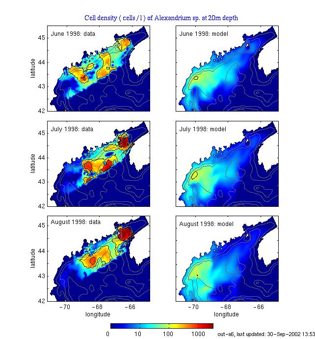
C = 0 | C = 0 | germ | cell98_a6.fli | cell98_a6.jpg |
|
same |
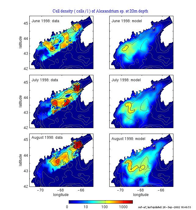
C = 0 | C = 0 | germ, growth, mort,
nutrient limitation |
cell98_a7.fli | cell98_a7.jpg |
|
same |
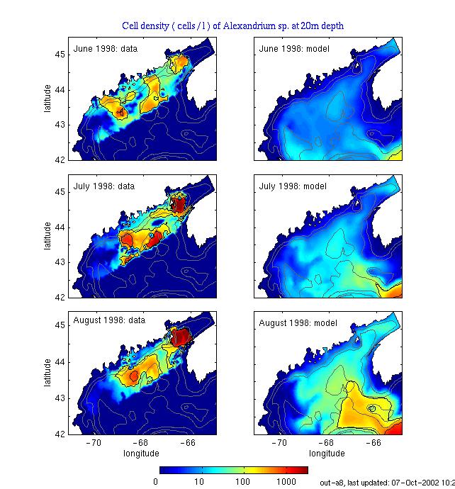
C = 10 | C = 10 | growth, mort, nutrient
limitation |
cell98_a8.fli | cell98_a8.jpg |
| sc98c1.fliis
the original Rich Signell's animation.
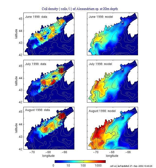
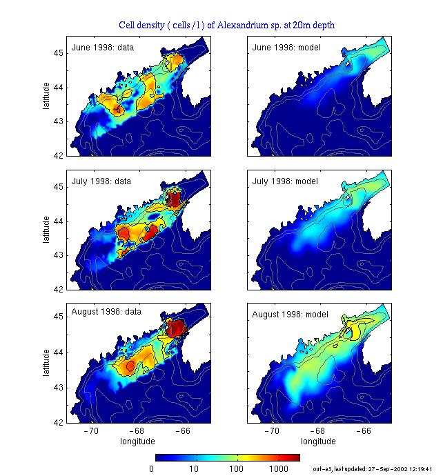
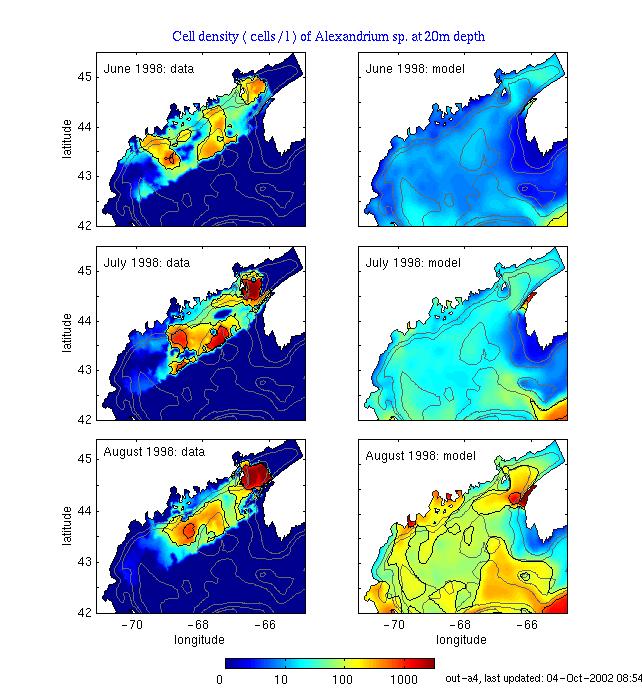
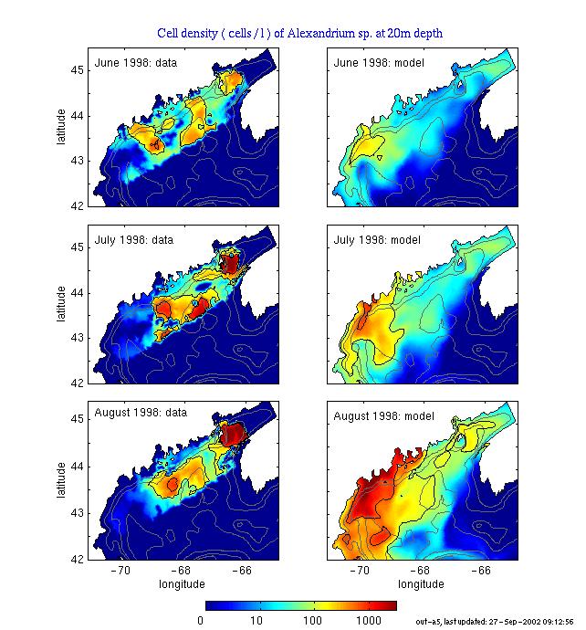
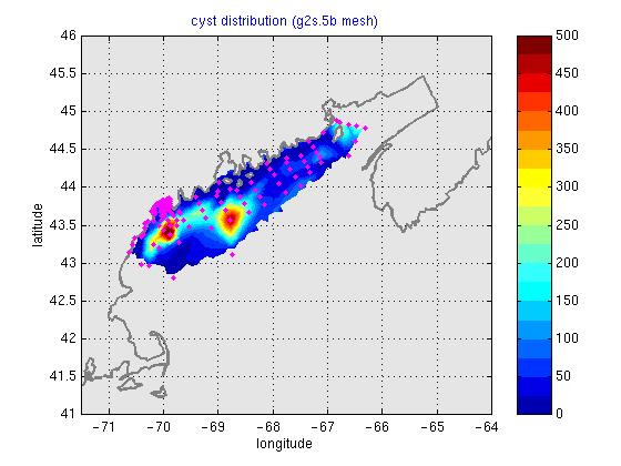
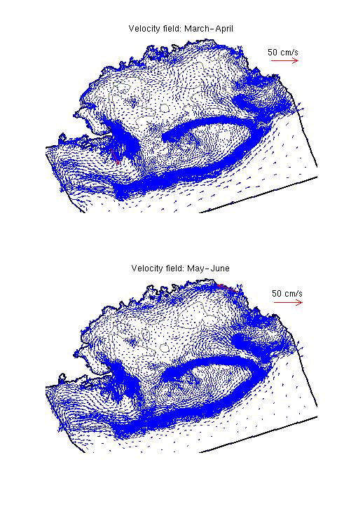
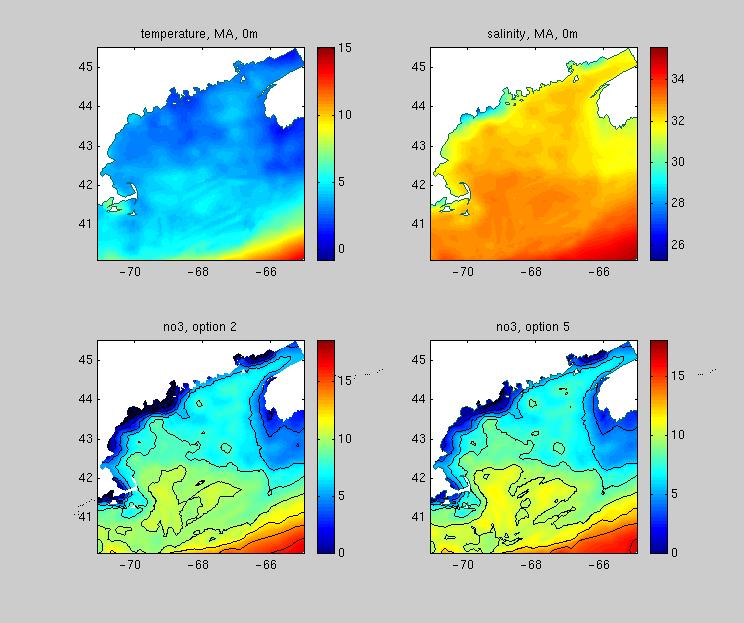
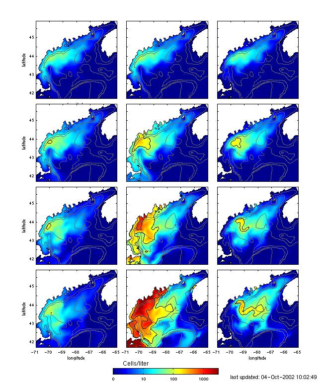
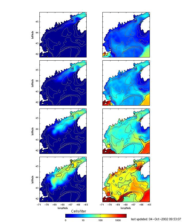
run a1. cell98_a1.fli Basic run. Initial cells concentration is et to zero, germination, growth and mortality included. Initial distribution of Alexandrium cysts in the upper 1 cm of bottom sediments, derived from a survey in October 1997, displayed in init_cyst.jpg. Two maxima in cysts distribution are clearly seen there: approximately between isobaths 75 and 150 m offshore of Kennebec River and Penobscot Bay. Also, an additional maximum may be tracked in the Bay of Fundy. Climatological velocity fields for two two bi-monthly periods are displayed here. Run starts on March 1, 1997 when the endogenous clock is on. run a3. cell98_a3.fli Initial cell concentration is set to zero, no germination, the only grows and mortality are included. There is a cell flux 10 cells/l flowing in through the open boundary in the Bay of Fundy. run a4. cell98_a4.fli Initial cell concentration is set to 10 cell/l; no germination, the only growth and mortality are included. There is a cell flux 10 cells/l flowing in through the open boundary in the Bay of Fundy. run a5. cell98_a5.fli Initial cells concentration is set to zero, germination, growth and mortality included. There is a cell flux 10 cells/l flowing in through the open boundary in the Bay of Fundy. run a6. cell98_a6.fli Initial cells concentration is set to zero, the only germination included. There is no cell flux flowing in through the open boundary in the Bay of Fundy. run a7. cell98_a7.fli Initial cells concentration is set to zero, germination, growth, mortality and nutrient limitation are included. NO3 distribution has been derived from the climatic temperature and salinity fields using a regression formula. Example of such distribution NO3 field received from the March-April climatology in case of two different regressions (2 and 5) is displayed here. run a8. cell98_a8.fli Initial cell concentration is set to 10 cell/l; no germination, the only growth, mortality, and nutrient limitation are included. There is a cell flux 10 cells/l flowing in through the open boundary in the Bay of Fundy. A composite of cell distribution for 3 model
runs: a6, a1, and a7 on May 15, June 15, July 15, and August
15 is presented in cell_model_a617.jpg.
A seperate plot displaying results of run a6 may
be found here: cell_model_a6.jpg.
A composite for runs 3, 4 is in
cell_model_a34.jpg.
|
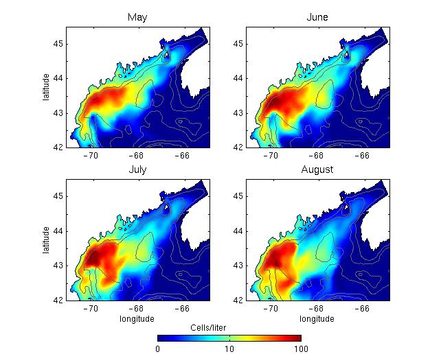
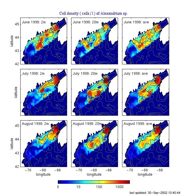
| Cell densities (number of cells / l)
of Alexandrium sp. at 2m, 20m, and the average of these two centered
on June 11, July 11, and August 11 1998 are shown here: cell98_data_ave.jpg.
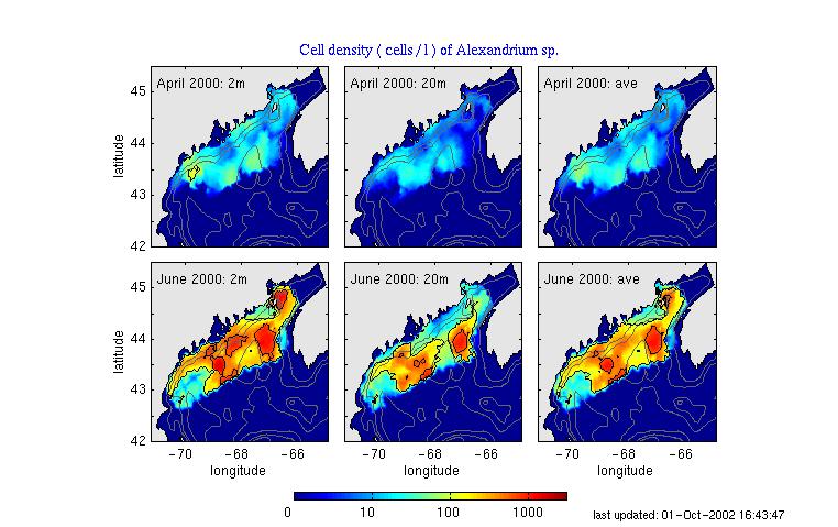
Cell densities for 2000 survey cruise centered on April 29 and June 9 are
shown in cell2000_data_ave.jpg.
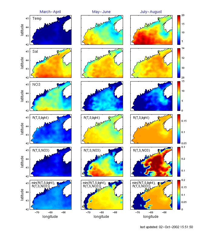
The 100 and 600 cells/l contour lines are given. A growth rate diagnosis based on the climatical March-April, May-June, and July-August bi-monthly fields is presented here: cell98_diagn.jpg. Notes on frames. Rows 1, 2: Temperature and salinity at the uppermost level. Row 3: NO3 field restored from the climatological temperature and salinity fields using a regression relation. Row 4: The growth rate (1/day) depending only on light limitation. Row 5: The growth rate (1/day) dependent only on nutrient limitation. Note on equations used to compute NO3 field and growth rates. NO3 = max(0,NO3'), NO3' = -144.8 - 0.38 * T + 4.75 * S (option 2) R-light = (G_max * G_fac + Gr) * tanh(G_eff * Rad/(G_max * G_fac + Gr)) - Gr , light limitation R-no3 = G_max * G_fac * NO3/(NO3 + aksn), NO3 limitation,
R = min(R-light, R-no3) - Graze, light and NO3 limitation
G_fac = T_fac * S_fac,
|